# Load packages using pacman (installs if missing, then loads).
pacman::p_load(ggplot2, dplyr, patchwork, purrr)

# A clean theme: light background, no grid lines.
# Note: "CMU Sans Serif" must be installed on your system to take effect.
theme <- theme_light(base_size = 10, base_family = "CMU Sans Serif") +
theme(panel.grid = element_blank())Simulating Publication Bias and Bayesian Learning
Overview
This document simulates a simple world in which:
- A population has a true mean \(\mu\) and standard deviation \(\sigma\).
- Researchers repeatedly run one-sample studies to estimate \(\mu\) and test \(H_0:\mu=0\) at \(\alpha=0.05\).
- A learner updates beliefs about \(\mu\) sequentially using Bayes’ rule under a normal-likelihood / known-SE approximation and a flat prior.
- Publication bias enters at the learning stage: insignificant findings are dropped with probability \(\rho\), so the learner often never sees them.
The main outputs are plots showing how the posterior mean and uncertainty evolve, and how publication bias distorts what the learner concludes.
Setup
Core simulation code
1) Generate a population with known parameters
# Create a population with a known mean (mu) and standard deviation (sigma).
# N_pop is large so that sampling variability mainly reflects "study sampling"
# rather than quirks of a small finite population.
make_population <- function(N_pop = 1e6, mu = 0.2, sigma = 1, seed = NULL) {
  if (!is.null(seed)) set.seed(seed)
  rnorm(N_pop, mean = mu, sd = sigma)
}
What’s going on?
- We treat the data-generating process as Normal for simplicity.
- You “know” the true \(\mu\) and \(\sigma\) because you set them.
- Each study will later draw a sample from this population.
2) Pick a sample size that attains target power
# Choose n to achieve target power for a two-sided one-sample t-test of mean vs 0.
# Here beta is POWER (e.g., 0.8), not Type II error.
choose_n_for_power <- function(mu, sigma = 1, alpha = 0.05, beta = 0.8) {
  # Standardized effect size relative to the null of 0.
  d <- abs(mu) / sigma

  # If mu = 0, there is no effect to detect, so power targeting is ill-posed.
  if (d == 0) stop("mu must be nonzero to target a positive power against H0: mu=0.")

  # power.t.test solves for n given delta (=mu), sd, alpha, and desired power.
  ceiling(power.t.test(
    delta = abs(mu),
    sd = sigma,
    sig.level = alpha,
    power = beta,
    type = "one.sample",
    alternative = "two.sided"
  )$n)
}
What’s going on?
- Power depends on the effect size \(|\mu|/\sigma\), the significance level \(\alpha\), and the sample size \(n\).
power.t.test()inRgives the approximate \(n\) needed for the desired power under a t-test model.
3) Run many studies
# Run many studies: each study draws n observations from the population,
# computes the sample mean and standard error, and runs a two-sided t-test vs mu0.
run_studies <- function(pop,
                        n_studies = 5000,
                        mu0 = 0,
                        alpha = 0.05,
                        n = NULL,
                        replace = TRUE,
                        seed = NULL) {
  if (!is.null(seed)) set.seed(seed)
  if (is.null(n)) stop("Provide n, or compute it using choose_n_for_power().")

  # Preallocate vectors for speed (avoid growing objects in a loop).
  est  <- numeric(n_studies)  # point estimate (sample mean)
  se   <- numeric(n_studies)  # estimated standard error
  tval <- numeric(n_studies)  # t-statistic
  pval <- numeric(n_studies)  # two-sided p-value

  for (i in seq_len(n_studies)) {
    # Each "study" samples n units from the population.
    samp <- sample(pop, size = n, replace = replace)

    # Sample statistics.
    m <- mean(samp)
    s <- sd(samp)

    # Estimate and its SE.
    est[i] <- m
    se[i]  <- s / sqrt(n)

    # Classical test statistic and p-value (two-sided).
    tval[i] <- (m - mu0) / se[i]
    pval[i] <- 2 * pt(-abs(tval[i]), df = n - 1)
  }

  # Return a tidy data frame of study-level outputs.
  data.frame(
    study_id = seq_len(n_studies),
    n = n,
    estimate = est,
    se = se,
    t = tval,
    p = pval,
    significant = (pval < alpha)
  )
}
What’s going on?
- Each row is a study.
- A study produces an estimate and a standard error.
- The significant indicator is based on the classical p-value threshold.
Learning with publication bias
Bayesian updating model
We use a deliberately naive model:
- Likelihood: \(\hat{\mu}_i \mid \mu \sim \mathcal{N}(\mu, \text{se}_i^2)\) for each study \(i\).
- Prior: flat (improper) prior over \(\mu\)
Under this model, the posterior after observing studies \(1,\dots,k\) is Normal with:
- precision \(P_k = \sum_{i=1}^k 1/\text{se}_i^2\)
- mean \(m_k = \frac{\sum_{i=1}^k \hat{\mu}_i/\text{se}_i^2}{\sum_{i=1}^k 1/\text{se}_i^2}\)
- sd \(s_k = 1/\sqrt{P_k}\)
Publication bias mechanism
The learner does not necessarily observe every study:
- If a study is significant, it is always observed.
- If a study is insignificant, it is dropped with probability \(\rho\).
- Dropped studies are skipped in the updating chain.
Show code
# Learn sequentially with a flat prior and normal likelihoods with known SE.
# Publication bias: insignificant studies are dropped with probability rho.
learn <- function(studies_df,
                  rho = 0,                 # P(drop | insignificant)
                  journal_alpha = 0.05,    # (kept for clarity; here significance uses studies_df$significant)
                  conf.int = TRUE,
                  conf.level = 0.5,
                  seed = NULL) {

  # ---- validation ----
  if (any(!is.finite(studies_df$estimate))) stop("Non-finite values found in `estimate`.")
  if (any(!is.finite(studies_df$se))) stop("Non-finite values found in `se`.")
  if (any(studies_df$se <= 0)) stop("All `se` must be > 0 for normal updating.")
  if (!is.numeric(rho) || length(rho) != 1 || rho < 0 || rho > 1) stop("rho must be a single number in [0, 1].")
  if (!is.numeric(journal_alpha) || length(journal_alpha) != 1 || journal_alpha <= 0 || journal_alpha >= 1) {
    stop("journal_alpha must be in (0, 1).")
  }
  if (!is.numeric(conf.level) || length(conf.level) != 1 || conf.level <= 0 || conf.level >= 1) {
    stop("conf.level must be in (0, 1).")
  }
  if (!is.null(seed)) set.seed(seed)

  # Ensure "time" order is study_id order.
  studies_df <- studies_df[order(studies_df$study_id), ]
  k <- nrow(studies_df)

  # ---- publication bias draw ----
  # For each study, draw a uniform random number u ~ U(0,1).
  # If the result is insignificant and u < rho, the study is dropped (never observed).
  u <- runif(k)
  dropped <- (!studies_df$significant) & (u < rho)
  used <- !dropped

  # ---- sequential updating ----
  post_mean <- numeric(k)
  post_sd   <- numeric(k)
  q25       <- numeric(k)
  q75       <- numeric(k)
  included_n <- integer(k)  # number of studies actually incorporated so far

  # Posterior precision and mean (under a flat prior).
  prec <- 0
  m <- 0

  for (i in seq_len(k)) {

    # Only update if the study is observed (not dropped).
    if (used[i]) {
      est <- studies_df$estimate[i]
      sei <- studies_df$se[i]
      wi  <- 1 / (sei^2)  # study precision: more precise studies get more weight

      # Combine old posterior (prec, m) with new likelihood contribution (wi, est).
      prec_new <- prec + wi
      m_new <- (prec * m + wi * est) / prec_new

      prec <- prec_new
      m <- m_new
    }

    # Summarize the posterior after processing study i (whether used or skipped).
    sd <- if (prec > 0) 1 / sqrt(prec) else Inf

    post_mean[i] <- if (prec > 0) m else NA_real_
    post_sd[i]   <- sd
    q25[i]       <- if (prec > 0) qnorm(0.25, mean = m, sd = sd) else NA_real_
    q75[i]       <- if (prec > 0) qnorm(0.75, mean = m, sd = sd) else NA_real_

    included_n[i] <- sum(used[seq_len(i)])
  }

  out <- data.frame(
    study_id       = studies_df$study_id,
    mean           = post_mean,
    sd             = post_sd,
    p25            = q25,
    p75            = q75,
    used_in_update = used,
    dropped        = dropped,
    n_included     = included_n
  )

  # Optional posterior interval (Normal approximation).
  if (conf.int) {
    a <- 1 - conf.level
    out$ci_lower <- ifelse(is.finite(out$sd),
                           qnorm(a / 2, mean = out$mean, sd = out$sd),
                           NA_real_)
    out$ci_upper <- ifelse(is.finite(out$sd),
                           qnorm(1 - a / 2, mean = out$mean, sd = out$sd),
                           NA_real_)
  }

  out
}
What’s going on?
- The posterior mean is a precision-weighted average of observed study estimates.
- Publication bias changes which estimates enter that average.
- The object
n_includedis useful because “study number” and “number of observed studies” can diverge under bias.
Example simulation
# True parameters
mu_true <- 0.5
sigma_true <- 1
alpha <- 0.05
beta  <- 0.8  # target power

# 1) Generate a large population
pop <- make_population(N_pop = 1e6, mu = mu_true, sigma = sigma_true, seed = 1)

# 2) Choose per-study sample size for target power
n_per_study <- choose_n_for_power(mu = mu_true, sigma = sigma_true,
                                 alpha = alpha, beta = beta)

# 3) Run a set of studies (no publication bias here; bias enters in learn()).
all_results <- run_studies(pop, n_studies = 1e3, mu0 = 0,
                           alpha = alpha, n = n_per_study, seed = 2)

# 4) Learn under different bias levels, using the same random seed so only rho varies.
no_bias        <- learn(all_results, rho = 0.0, seed = 123)
rho_20pct_bias <- learn(all_results, rho = 0.2, seed = 123)
rho_50pct_bias <- learn(all_results, rho = 0.5, seed = 123)

# Stack the learning paths into one data frame for plotting.
studies <- bind_rows(
  `0% bias`  = no_bias,
  `20% bias` = rho_20pct_bias,
  `50% bias` = rho_50pct_bias,
  .id = "bias_level"
)
Plots
Posterior mean over time
p1 <- ggplot(studies, aes(x = study_id, y = mean, color = bias_level, fill = bias_level)) +
  scale_x_continuous("Study number (in order of publication)", breaks = seq(0, 1000, by = 200)) +
  scale_y_continuous("Posterior estimate μ") +
  guides(
    color = guide_legend(title = "P(Drop | Insignificant)"),
    fill  = guide_legend(title = "P(Drop | Insignificant)")
  ) +
  # The true mu is a reference line: where the posterior *should* converge without bias.
  geom_hline(yintercept = mu_true, linetype = "dashed", color = "black") +
  geom_line() +
  # Ribbon shows the posterior interval (here conf.level = 0.5 by default).
  geom_ribbon(aes(ymin = ci_lower, ymax = ci_upper), alpha = 0.3) +
  theme +
  theme(legend.position = "bottom")

p1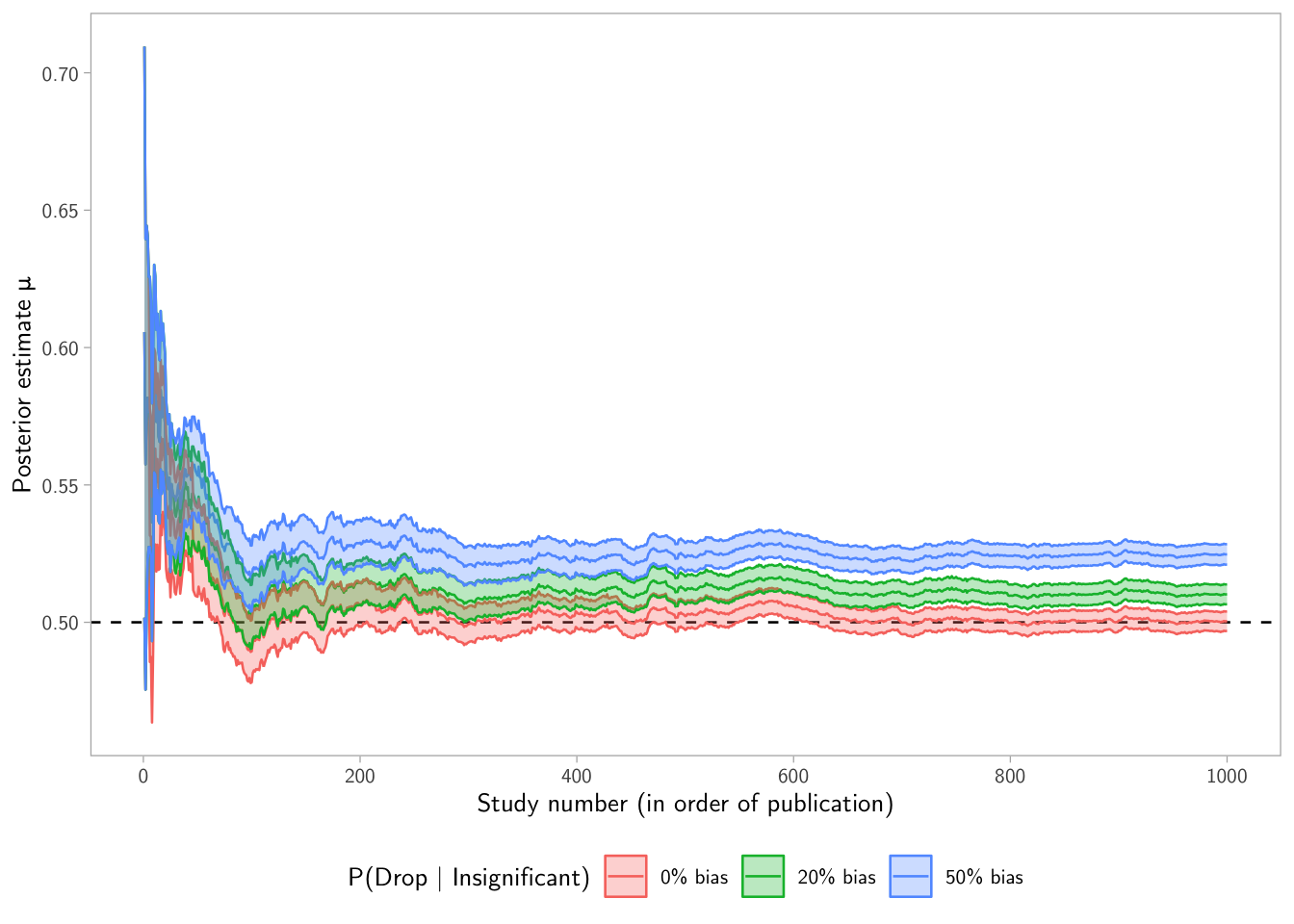
Interpretation tip: if publication bias suppresses nulls, the posterior mean can drift away from the truth because the learner overweights “exciting” estimates.
Posterior uncertainty (sd) over time
p2 <- ggplot(studies, aes(x = study_id, y = sd, color = bias_level)) +
  scale_x_continuous("Study number", breaks = seq(0, 1000, by = 200)) +
  # sd shrinks fast early on, so a log scale is often easier to read.
  scale_y_log10("Posterior σ (log-scaled)") +
  guides(color = "none") +
  geom_line() +
  theme +
  theme(legend.position = "bottom")

p2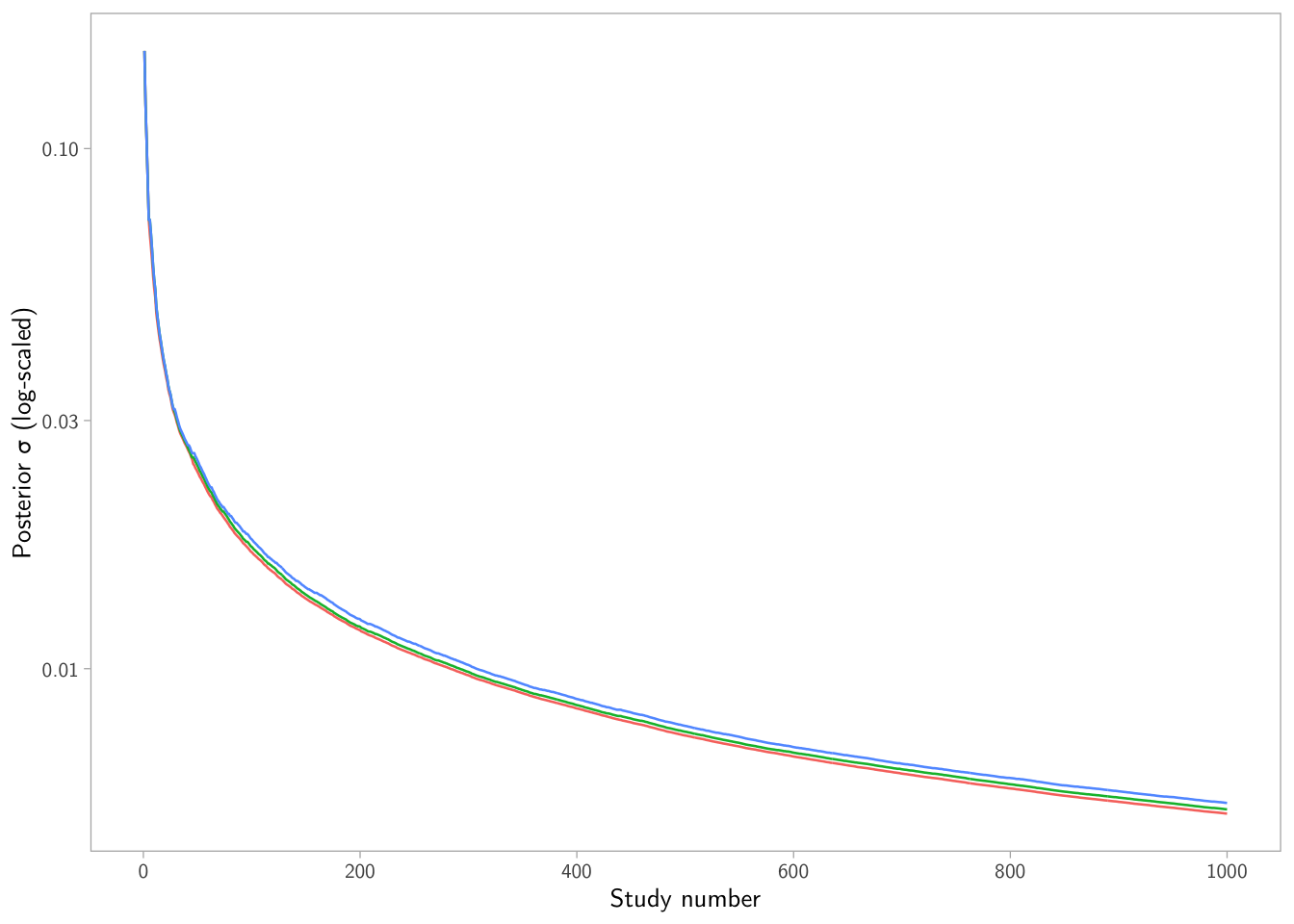
What’s going on? When the learner sees fewer studies (because nulls are dropped), the precision accumulates more slowly, so uncertainty can stay larger for longer.
Cumulative number of published null results
p3 <- studies |>
  left_join(all_results, by = "study_id") |>
  # "published_null" is 1 if the result is null and not dropped; 0 otherwise.
  # - If significant: 0 (not a null result)
  # - If insignificant and not dropped: 1
  # - If insignificant and dropped: 0
  mutate(published_null = ifelse(significant, 0, 1) - ifelse(dropped, 1, 0)) |>
  mutate(nulls_observed = cumsum(published_null), .by = bias_level) |>
  ggplot(aes(x = study_id, y = nulls_observed, color = bias_level)) +
  scale_x_continuous("Study number (in order of publication)", breaks = seq(0, 1000, by = 200)) +
  scale_y_continuous("Cum. # of published null results") +
  guides(color = "none") +
  geom_line() +
  theme +
  theme(legend.position = "bottom")

p3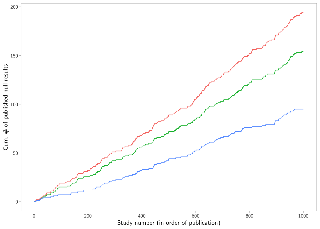
What’s going on? This plot makes the selection mechanism visible: higher \(\rho\) implies fewer published nulls accumulate.
Distribution of posterior means after all studies
posterior <- studies |>
  group_by(bias_level) |>
  slice_max(order_by = study_id, n = 1, with_ties = FALSE) |>
  select(bias_level, mean, sd, n_included)

p4 <- map(posterior$bias_level, function(bias) { rnorm(1e4, mean = posterior$mean[posterior$bias_level == bias], sd = posterior$sd[posterior$bias_level == bias]) }) |>
  set_names(posterior$bias_level) |>
  bind_rows(.id = "bias_level") |>
  tidyr::pivot_longer(cols = everything(), names_to = "bias_level", values_to = "mean") |>
  ggplot(aes(x = mean, fill = bias_level)) +
  scale_x_continuous("Posterior mean estimate after all studies") +
  scale_y_continuous("Density") +
  guides(fill = "none") +
  geom_vline(xintercept = mu_true, linetype = "dashed", color = "black") +
  geom_density(alpha = 0.5) +
  theme + theme(legend.position = "bottom")

p4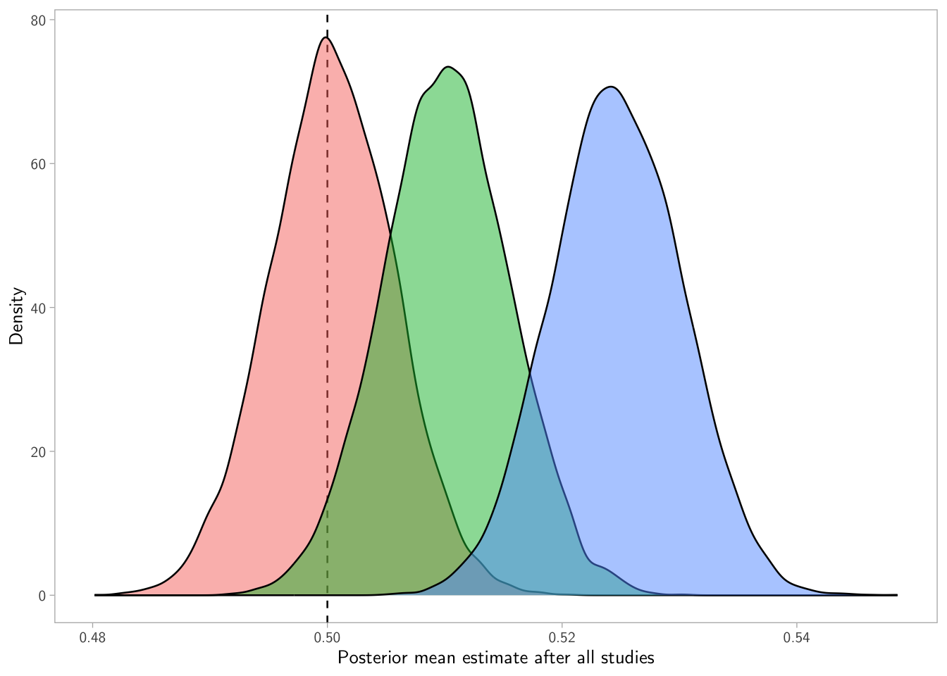
What’s going on? Each bias level produces a different terminal posterior mean, because each learning path filters evidence differently.
Combined figure
(p1 + p2) / (p3 + p4) +
  plot_layout(guides = "collect") &
  theme(legend.position = "bottom")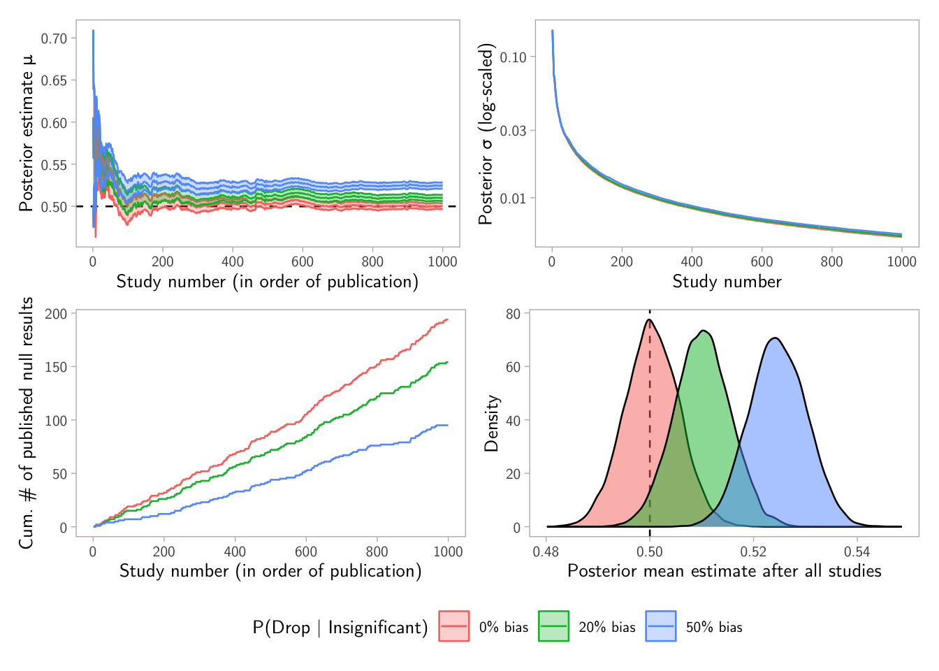
More simulations
Show code
make_dashboard <- function(mu_true,
                           sigma_true,
                           alpha = 0.05,
                           beta  = 0.8,
                           rho   = c(0, 0.2, 0.5),
                           n_studies = 1000,
                           N_pop = 1e6,
                           mu0 = 0,
                           conf.level = 0.5,
                           seed_pop = 1,
                           seed_studies = 2,
                           seed_learn = 123,
                           base_theme = theme_light(base_size = 14, base_family = "CMU Sans Serif") +
                             theme(panel.grid = element_blank()),
                           legend_title = "P(Reject | Insignificant)") {
  # Dependencies are assumed loaded by caller (ggplot2, dplyr, patchwork, purrr)
  # but we’ll reference explicitly where needed to avoid ambiguity.
  stopifnot(is.numeric(mu_true), length(mu_true) == 1)
  stopifnot(is.numeric(sigma_true), length(sigma_true) == 1, sigma_true > 0)
  stopifnot(is.numeric(alpha), length(alpha) == 1, alpha > 0, alpha < 1)
  stopifnot(is.numeric(beta),  length(beta)  == 1, beta  > 0, beta  < 1)
  stopifnot(is.numeric(n_studies), length(n_studies) == 1, n_studies >= 2)
  stopifnot(is.numeric(N_pop), length(N_pop) == 1, N_pop >= 1000)
  stopifnot(is.numeric(rho), all(rho >= 0 & rho <= 1))

  # Greek letters
  mu_chr <- "\u03BC"  # μ
  sd_chr <- "\u03C3"  # σ

  # 1) Population
  pop <- make_population(N_pop = N_pop, mu = mu_true, sigma = sigma_true, seed = seed_pop)

  # 2) Per-study n for desired power
  n_per_study <- choose_n_for_power(mu = mu_true, sigma = sigma_true, alpha = alpha, beta = beta)

  # 3) Run studies (no publication bias here)
  all_results <- run_studies(pop,
                            n_studies = n_studies,
                            mu0 = mu0,
                            alpha = alpha,
                            n = n_per_study,
                            seed = seed_studies)

  # 4) Learn under different publication-bias strengths
  rho <- sort(unique(rho))
  rho_labels <- paste0(round(100 * rho), "% bias")
  names(rho) <- rho_labels

  learned_list <- purrr::imap(rho, function(r, lab) {
    learn(all_results, rho = r, journal_alpha = alpha, conf.level = conf.level, seed = seed_learn)
  })

  studies <- dplyr::bind_rows(learned_list, .id = "bias_level") |>
    dplyr::mutate(
      bias_level = factor(bias_level, levels = rho_labels),
      rho_value  = rep(rho, each = n_studies)
    )

  # ---- P1: posterior mean path + ribbon ----
  p1 <- ggplot2::ggplot(studies, ggplot2::aes(x = study_id, y = mean, color = bias_level, fill = bias_level)) +
    ggplot2::scale_x_continuous("Study number",
                                breaks = seq(0, n_studies, by = max(1, floor(n_studies / 5)))) +
    ggplot2::scale_y_continuous(paste0("Post. estimate ", mu_chr)) +
    ggplot2::guides(
      color = ggplot2::guide_legend(title = legend_title),
      fill  = ggplot2::guide_legend(title = legend_title)
    ) +
    ggplot2::geom_hline(yintercept = mu_true, linetype = "dashed", color = "black") +
    ggplot2::geom_line() +
    ggplot2::geom_ribbon(ggplot2::aes(ymin = ci_lower, ymax = ci_upper), alpha = 0.3, color = NA) +
    base_theme +
    ggplot2::theme(legend.position = "bottom")

  # ---- P2: posterior sd path (log scale) ----
  p2 <- ggplot2::ggplot(studies, ggplot2::aes(x = study_id, y = sd, color = bias_level)) +
    ggplot2::scale_x_continuous("Study number",
                                breaks = seq(0, n_studies, by = max(1, floor(n_studies / 5)))) +
    ggplot2::scale_y_log10(paste0("Post. ", sd_chr, " (log-scaled)")) +
    ggplot2::guides(color = "none") +
    ggplot2::geom_line() +
    base_theme +
    ggplot2::theme(legend.position = "bottom")

  # ---- P3: cumulative published nulls ----
  p3 <- studies |>
    dplyr::left_join(all_results, by = "study_id") |>
    dplyr::mutate(
      published_null = ifelse(significant, 0, 1) - ifelse(dropped, 1, 0),
      nulls_observed = cumsum(published_null),
      .by = bias_level
    ) |>
    ggplot2::ggplot(ggplot2::aes(x = study_id, y = nulls_observed, color = bias_level)) +
    ggplot2::scale_x_continuous("Study number",
                                breaks = seq(0, n_studies, by = max(1, floor(n_studies / 5)))) +
    ggplot2::scale_y_continuous("Cum. # of published null results") +
    ggplot2::guides(color = "none") +
    ggplot2::geom_line() +
    base_theme +
    ggplot2::theme(legend.position = "bottom")

  # ---- P4: posterior distributions after final study ----
  posterior <- studies |>
    dplyr::group_by(bias_level) |>
    dplyr::slice_max(order_by = study_id, n = 1, with_ties = FALSE) |>
    dplyr::ungroup() |>
    dplyr::select(bias_level, mean, sd, n_included)

  draws <- purrr::map(posterior$bias_level, function(bias) {
    rnorm(1e4,
          mean = posterior$mean[posterior$bias_level == bias],
          sd   = posterior$sd[posterior$bias_level == bias])
  }) |>
    rlang::set_names(posterior$bias_level) |>
    dplyr::bind_rows(.id = "bias_level") |>
    tidyr::pivot_longer(everything(), names_to = "bias_level", values_to = "mean")

  p4 <- ggplot2::ggplot(draws, ggplot2::aes(x = mean, fill = bias_level)) +
    ggplot2::scale_x_continuous(paste0("Post. distribution of μ")) +
    ggplot2::scale_y_continuous("Density") +
    ggplot2::guides(fill = "none") +
    ggplot2::geom_vline(xintercept = mu_true, linetype = "dashed", color = "black") +
    ggplot2::geom_density(alpha = 0.5) +
    base_theme +
    ggplot2::theme(legend.position = "bottom")

  dashboard <- (p1 + p2) / (p3 + p4) +
    patchwork::plot_layout(guides = "collect") &
    ggplot2::theme(legend.position = "bottom")

  # Return plot, plus useful internals
  list(
    plot = dashboard,
    n_per_study = n_per_study,
    all_results = all_results,
    learned = studies
  )
}
What’s going on? This function wraps the whole simulation and plotting process, allowing you to easily generate dashboards for different parameter settings. You can call it with different mu_true, sigma_true, rho, etc. to see how the learning dynamics change.
\(\rho = (0~0.1~0.5)\) and \(\beta = 0.9\) example
result <- make_dashboard(mu_true = 0.5, sigma_true = 1, alpha = 0.05, beta = 0.9, rho = c(0, 0.1, 0.5), n_studies = 1000, N_pop = 1e6)

result$plot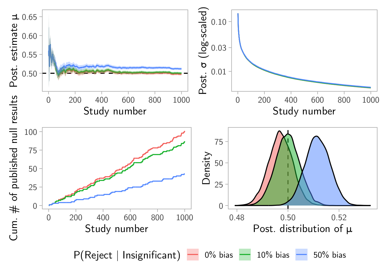
\(\rho = (0~0.5~0.8)\) and \(\beta = 0.2\) example
result <- make_dashboard(mu_true = 0.5, sigma_true = 1, alpha = 0.05, beta = 0.2, rho = c(0, 0.5, 0.8), n_studies = 1000, N_pop = 1e6)

result$plot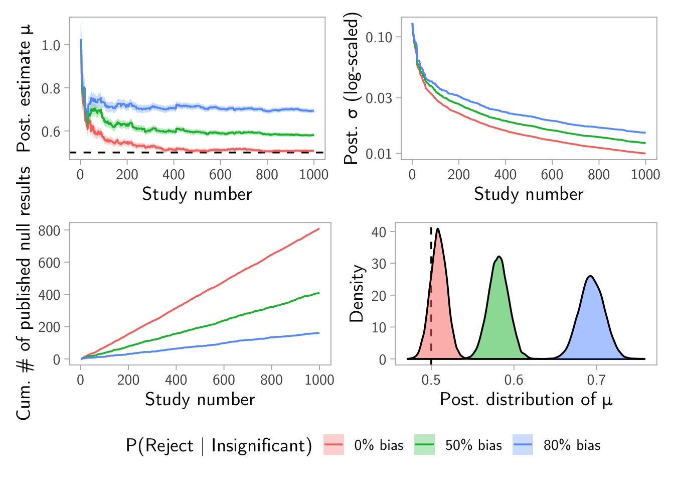
Notes and extensions
- Enable custom “selection functions” instead of just a fixed \(\rho\). For example, make \(\rho\) depend on the p-value and/or the estimate size.
- Make power heterogeneous across studies and see how naive learning is affected when the learner assumes a fixed \(n\) and \(\sigma\).
- Once heterogeneity is introduced, the learner would need to model it.